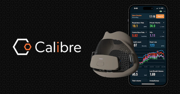
I recently picked up a Calibre Biometric Tracker. It’s essentially a face mask that tracks airflow and composition during exercise, allowing you to do cardiopulmonary exercise testing at home.
Initially I was skeptical, but the device has been demonstrated to be pretty accurate at a fraction of the cost of a full “metabolic cart”, and as a passionate VO2max tracker being able to derive “accurate” numbers was a really interesting proposition (and makes the nerdy work cycling group chat even nerdier).
So when the device finally arrived from America, I couldn’t wait to try it out. Despite a big run and gym effort earlier that day meaning I knew the numbers wouldn’t be ideal (excuses already?) but I loaded up a ramp test on Zwift and got pedaling until the legs got so heavy I could pedal no more.
Once I’d managed to recover, I had a look at the data. The mask slipped a couple of times due to my poor fitting, so it’s probably not as accurate as it could be, but it generated a lot of numbers:
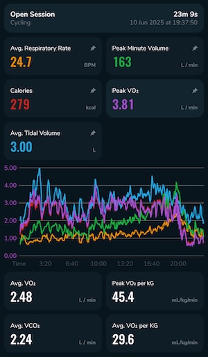
But what does this mean? The Calibre app does extract some numbers for you, but I’m far more used to seeing the classic nine-panel plot and interpreting that:
How can we get the data out of Calibre and into that format? Obviously there’s an R package for that in the form of {spiro} which generates and analyses such plots, but sadly spiro doesn’t yet import from Calibre.

Calibre spits out a CSV file that can be downloaded from the portal. However it doesn’t include either heart rate data or load, so we’ll also need to get the workout FIT file from Zwift, and combine the two.
The following function does this by comparing the timestamps:
spiro_get_calibre <- function(calibre_file,
                              zwift_file,
                              birthday) {

  # Step 1: Get info from Calibre ####
  raw <- utils::read.csv(calibre_file, stringsAsFactors = FALSE)

  # Extract metadata (first 20 rows of Session Data column)
  meta_rows <- raw[1:20, c("Session.Data", "X")]
  meta_keys <- tolower(gsub("[[:punct:][:space:]]+", "", meta_rows$Session.Data))
  meta_vals <- meta_rows$X
  names(meta_vals) <- meta_keys

  # Extract fields
  extract_meta <- function(patterns) {
    match <- grep(paste(patterns, collapse = "|"), names(meta_vals), value = TRUE)
    if (length(match) > 0) return(meta_vals[[match[1]]])
    return(NA)
  }

  bodymass <- as.numeric(extract_meta(c("weight", "bodyweightkg")))
  starttime <- lubridate::mdy_hms(extract_meta(c("utcdatetime"))) # Note US format

  # Filter data rows
  data <- raw[!is.na(suppressWarnings(as.numeric(raw[["Timer..s."]]))), ]
  data[] <- lapply(data, function(x) suppressWarnings(as.numeric(as.character(x))))

  df_c <- data.frame(
    time   = data[["Timer..s."]],
    VO2    = data[["VO2..slpm."]]*1000, # L > mls
    VCO2   = data[["VCO2..slpm."]]*1000,
    RR     = data[["Respiratory.Rate..breaths.min."]],
    VT     = data[["Tidal.Volume..l."]],
    VE     = data[["Minute.Volume..l.min."]],
    #HR     = data[["HR..bpm."]], # Get from zwift
    #load   = NA,                 # Get from zwift
    PetO2  = (760-47)*(data[["Exhaled.O2...."]]/100), # %O2 to FeO2 to mmHg
    PetCO2 = (760-47)*(data[["Exhaled.CO2...."]]/100) # Assumes 1atm of pressure
  )

  # Step 2: Get info from Zwift ####
  zwift_raw <- FITfileR::records(FITfileR::readFitFile(zwift_file))

  # Extract variables
  df_z <- data.frame(
    timestamp = zwift_raw[["timestamp"]],
    HR        = zwift_raw[["heart_rate"]],
    load      = zwift_raw[["target_power"]]
  )

  # Step 3: Combine and tidy ####

  # Convert seconds to timestamp in calibre
  # May need to check everything is UTC?
  df_c$timestamp <- starttime + as.difftime(df_c$time - 1, units = "secs")
  df_c2 <- df_c[ , !(names(df_c) %in% "time")]

  # Join on timestamp, remove lines with no load
  df <- merge(df_z, df_c2, by = "timestamp", all = TRUE)
  df <- df[!is.na(df$load) & df$load > 0, ]

  # Convert back to seconds from start
  df$time <- as.numeric(df$timestamp - min(df$timestamp, na.rm = TRUE))
  df <- df[, !(names(df) %in% "timestamp")]

  # Remove unrealistic values
  df$HR[df$HR == 0] <- NA
  df <- df[!is.na(df$time), ]

  # Extract data frame extras
  info <- data.frame(
    # These are in {spiro} but not provided by the Calibre device
    #name = name,
    #surname = surname,
    #birthday = birthday,
    #sex = sex,
    #height = height,
    # Things we do know (and need for plotting)
    bodymass = bodymass,
    birthday = lubridate::dmy(birthday)
  )

  # Add necessary attributes
  attr(df, "info") <- info
  class(df) <- c("spiro", "data.frame")
  return(df)
}
Now we can process that data using the rest of the {spiro} library:
library(spiro)
dt_imported <- spiro_get_calibre(calibre_file, zwift_file, birthday)
# Find the exercise protocol
ptcl <- get_protocol(dt_imported)
dt_ptcl <- add_protocol(data = dt_imported, protocol = ptcl)
# add data calculated from body mass
dt_out <- add_bodymass(data = dt_ptcl)
# calculate additional variables
dt_out$RER <- dt_out$VCO2 / dt_out$VO2
dt_out$RER[which(is.na(dt_out$RER))] <- NA
dt_out <- calo(data = dt_out)
# save raw data as attribute
attr(dt_out, "raw") <- dt_imported
# plot the data
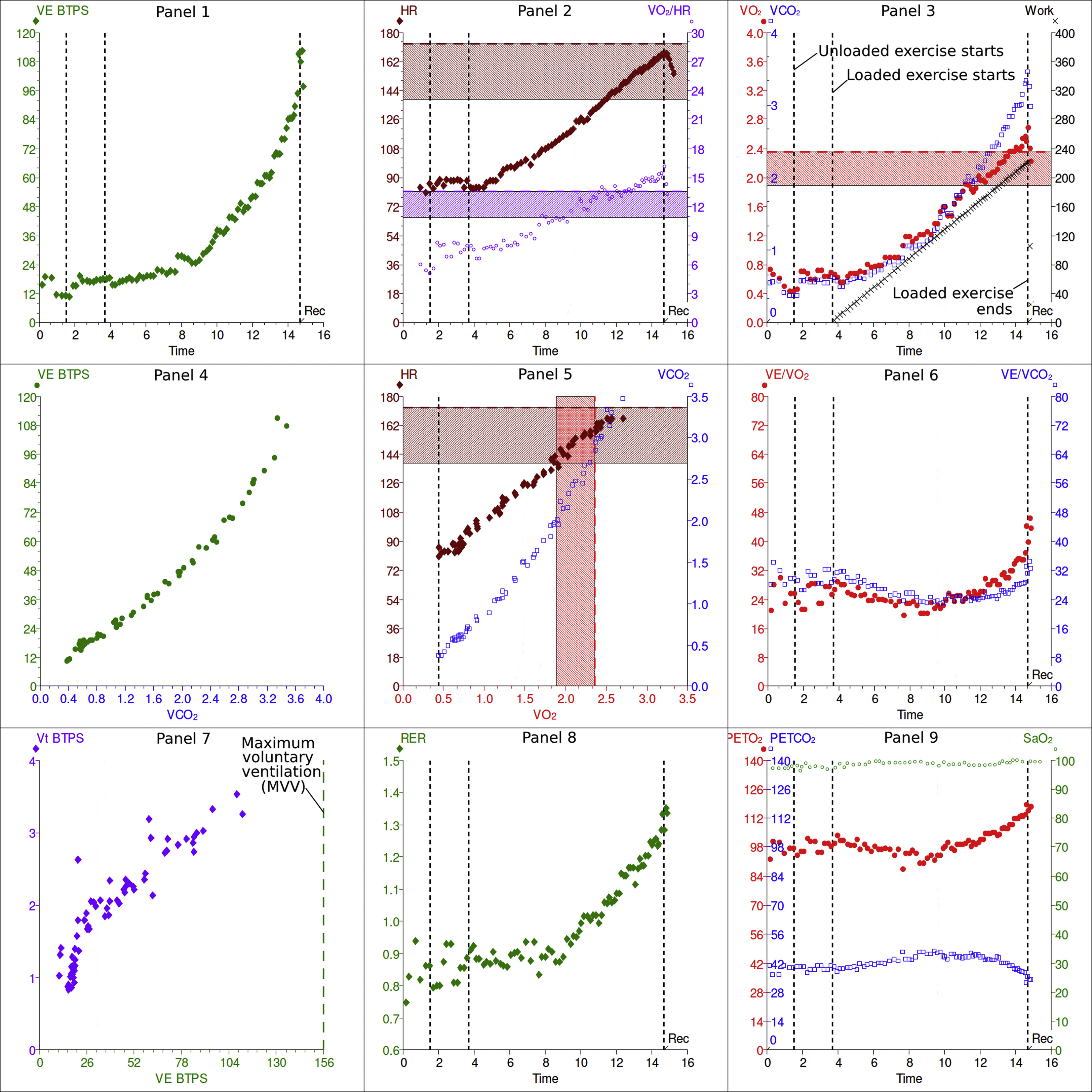
spiro_plot(dt_out)Which results in a lovely nine-panel plot:
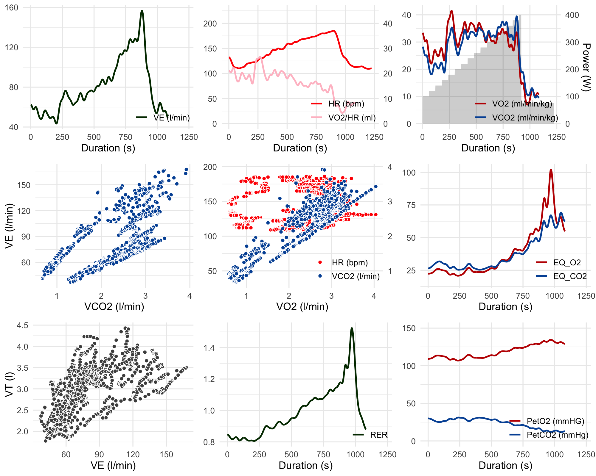
Yes, it looks a bit abnormal - in particular VO2peak occurred before the end of the test, and oxygen pulse tailed off after ~8mins in - however I think that’s due to the mask falling off my face at this point rather than having severe cardiac limitation! I’ll have another attempt at the ramp test after I finish this training block for the Dragon Ride but hopefully this code will help other Calibre owners make use of their data in the meantime.