In case it’s completely passed you by, The Traitors has become a bit of a cultural phenomenon in the UK. Now in it’s fourth series, the reality-TV-game show (based on the Dutch show De Verraders, which in turn is based on the party game Mafia) features a small group of “traitors” trying to disrupt, murder, and banish the “faithful” until just they remain.

The problem is that’s it’s starting to look like people of colour, and in particular black or brown players, are being voted out or murdered much earlier into the game than the (majority) white contestants. Multiple news agencies have highlighted the risk of unconscious bias underlying this phenomena, and the risks involved in such ways of thinking outside of the game.

On the Traitors subreddit, a social scientist ran the numbers to see if this really is the case. I reached out to them for a copy of their dataset, and I’ve updated it to the finale of season 4 (sorry for any spoilers). They manually coded players by their photos where identified ethnicity was not available, which is potentially the major weakness in this analysis, but that aside we can investigate this phenomenon statistically.

Build a dataset

library(tidyverse)
library(janitor)
library(survival)
library(survminer)
library(brms)
library(tidybayes)

# Use cmdstanr for speed
options(brms.backend = "cmdstanr")

# Import ####
raw <- read_csv("traitors_uk.csv") %>% clean_names()

We need to start by censoring and deriving relevant variables. When I initially started this episode 4 was still ongoing, so I’ve written in the ability to right-censor players who are still in the game:

dat <- raw %>%
  mutate(
    season = as.integer(season),
    age = as.numeric(age),
    bb = as.integer(black_brown),
    gender = factor(gender),
    
    exit_method = as.character(exit_method),
    exit_episode = as.integer(exit_episode),
    
    started_as = as.character(started_as),
    started_traitor = as.integer(started_as == "Traitor"),
    
    recruit_ep = as.integer(traitor_recruit_episode)
  )

# Find last episode to work out who is still in the game
last_ep_by_season <- dat %>%
  group_by(season) %>%
  summarise(last_ep = max(exit_episode, na.rm = TRUE), .groups = "drop")

# Censor players
dat <- dat %>%
  left_join(last_ep_by_season, by = "season") %>%
  mutate(
    time = if_else(!is.na(exit_episode), exit_episode, last_ep),
    
    # "Any elimination" event:
    event_any = as.integer(exit_method %in% c("Banished", "Murdered", "Eliminated")),
    
    #   Event_any = 1 if banished/murdered/eliminated else 0
    # i.e. for winners/runner-up/still-in-game: event_any = 0
    event_any = if_else(is.na(event_any), 0L, event_any),
    
    age_z = as.numeric(scale(age))
  )

# Checks
# dat %>% count(season, in_game)
# dat %>% count(exit_method, sort = TRUE)
# dat %>% summarise(
#   n = n(),
#   n_bb = sum(bb == 1, na.rm = TRUE),
#   n_missing_bb = sum(is.na(bb))
# )

We can now turn this into “survival” by creating a person–episode (discrete time) dataset. We’ll expand each contestant into one row per episode survived, with \(y = 1\) at the elimination episode (if event), else all zeros. We’ll also create a time-varying traitor status traitor_t:

make_person_episode <- function(dat, max_episode_cap = 12) {
  dat %>%
    filter(!is.na(bb), !is.na(age_z), !is.na(time)) %>%
    mutate(
      id = row_number(),
      time = pmin(as.integer(time), max_episode_cap)
    ) %>%
    select(id, season, contestant, time, event_any, exit_method,
           bb, age_z, gender, started_traitor, recruit_ep) %>%
    group_by(id) %>%
    summarise(
      across(-time, first),
      episode = list(seq_len(first(time))),
      .groups = "drop"
    ) %>%
    unnest(episode) %>%
    group_by(id) %>%
    mutate(
      y_any = as.integer(episode == max(episode) & event_any == 1L),
      
      # time-varying traitor status:
      traitor_t = as.integer(
        started_traitor == 1L |
          (!is.na(recruit_ep) & episode >= recruit_ep)
      )
    ) %>%
    ungroup()
}

pe <- make_person_episode(dat)

# Checks
# pe %>% count(episode) %>% print()
# pe %>% count(season, episode) %>% print(n = 50)

Risk of leaving the show (by any means)

We can demonstrate the unadjusted difference between groups using Kaplain-Meier curves. The probability of a black or brown contestent surviving does seem lower than contestents of other ethnicities, although the confidence intervals in these estimates overlap:

# Convert back to one row per contestant (id) for {survival}
subj <- pe %>%
  group_by(id) %>%
  summarise(
    bb = first(bb),
    season = first(season),
    age_z = first(age_z),
    gender = first(gender),
    started_traitor = first(started_traitor),
    time = max(episode),                    # last observed episode
    event_any = max(y_any),                 # 1 if eliminated at last episode, else 0
    .groups = "drop"
  ) %>%
  filter(!is.na(bb), !is.na(time), !is.na(event_any)) %>% 
  filter(complete.cases(bb, time, event_any, season))

subj %>% count(bb)

# A tibble: 2 × 2
     bb     n
  <int> <int>
1     0    64
2     1    27

km_fit <- survfit(Surv(time, event_any) ~ bb, data = subj)

ggsurvplot(km_fit, data = subj,
           risk.table = TRUE, conf.int = TRUE,
           xlab = "Episode", ylab = "Survival probability",
           legend.labs = c("Non-BB", "BB"))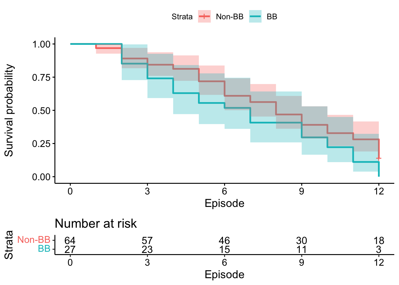

This seems to be a fairly consistent finding across series:

ggsurvplot_facet(km_fit, subj, 
                 facet.by = "season", 
                 nrow = 2,
                 conf.int = TRUE, risk.table = FALSE)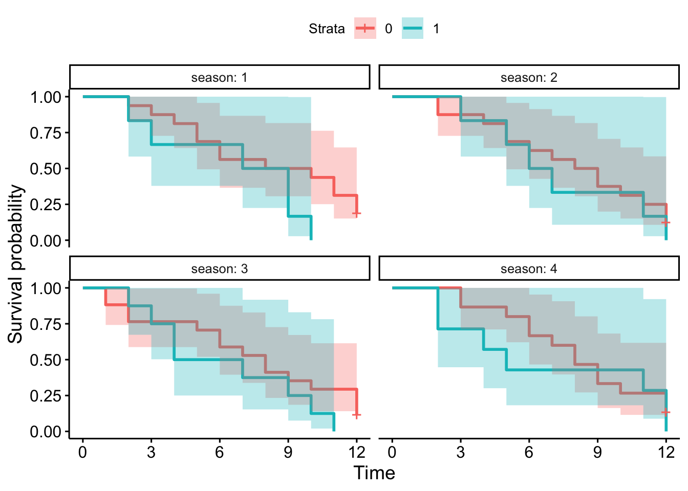

The most straightforward way of assessing this is using a Cox propotional-hazards model. We can start with a simple, unadjusted model - risk of leaving the show by any means is purely dependent on skin colour:

cox_unadj <- coxph(Surv(time, event_any) ~ bb, data = subj)
summary(cox_unadj)

Call:
coxph(formula = Surv(time, event_any) ~ bb, data = subj)

  n= 91, number of events= 82 

     coef exp(coef) se(coef)     z Pr(>|z|)  
bb 0.4980    1.6454   0.2388 2.085    0.037 *
---
Signif. codes:  0 '***' 0.001 '**' 0.01 '*' 0.05 '.' 0.1 ' ' 1

   exp(coef) exp(-coef) lower .95 upper .95
bb     1.645     0.6077      1.03     2.628

Concordance= 0.548  (se = 0.029 )
Likelihood ratio test= 4.1  on 1 df,   p=0.04
Wald test            = 4.35  on 1 df,   p=0.04
Score (logrank) test = 4.44  on 1 df,   p=0.04

This simple model suggests that being black or brown leads to an increased hazard of elimination of 1.65 (95% confidence intervals 1.03-2.67, p = 0.037), i.e. 65% higher risk of leaving the game for any reason.

But we can also try adjusting this for the contestent’s gender, age, traitor status, and season:

cox_adj <- coxph(Surv(time, event_any) ~ bb + season + age_z + gender + started_traitor, data = subj)
summary(cox_adj)

Call:
coxph(formula = Surv(time, event_any) ~ bb + season + age_z + 
    gender + started_traitor, data = subj)

  n= 90, number of events= 81 
   (1 observation deleted due to missingness)

                    coef exp(coef) se(coef)      z Pr(>|z|)    
bb               0.56386   1.75744  0.24842  2.270 0.023221 *  
season           0.02775   1.02814  0.09989  0.278 0.781128    
age_z            0.42290   1.52638  0.12068  3.504 0.000458 ***
genderM          0.08743   1.09136  0.23952  0.365 0.715099    
started_traitor -0.42967   0.65072  0.33138 -1.297 0.194763    
---
Signif. codes:  0 '***' 0.001 '**' 0.01 '*' 0.05 '.' 0.1 ' ' 1

                exp(coef) exp(-coef) lower .95 upper .95
bb                 1.7574     0.5690    1.0800     2.860
season             1.0281     0.9726    0.8453     1.250
age_z              1.5264     0.6551    1.2049     1.934
genderM            1.0914     0.9163    0.6825     1.745
started_traitor    0.6507     1.5368    0.3399     1.246

Concordance= 0.63  (se = 0.037 )
Likelihood ratio test= 17.17  on 5 df,   p=0.004
Wald test            = 18.18  on 5 df,   p=0.003
Score (logrank) test = 18.81  on 5 df,   p=0.002

This model suggests that age is the strongest risk factor for elimination from the game (p < 0.001), with being black or brown second (hazard ratio 1.78 ,95% confidence intervals 1.09-2.89, p = 0.021).