Code
library(tidyverse)
library(lubridate)
library(brms)
library(posterior)Looks like resident doctors are going back on strike next month. This latest round of industrial action is part of a long running campaign for full pay restoration.
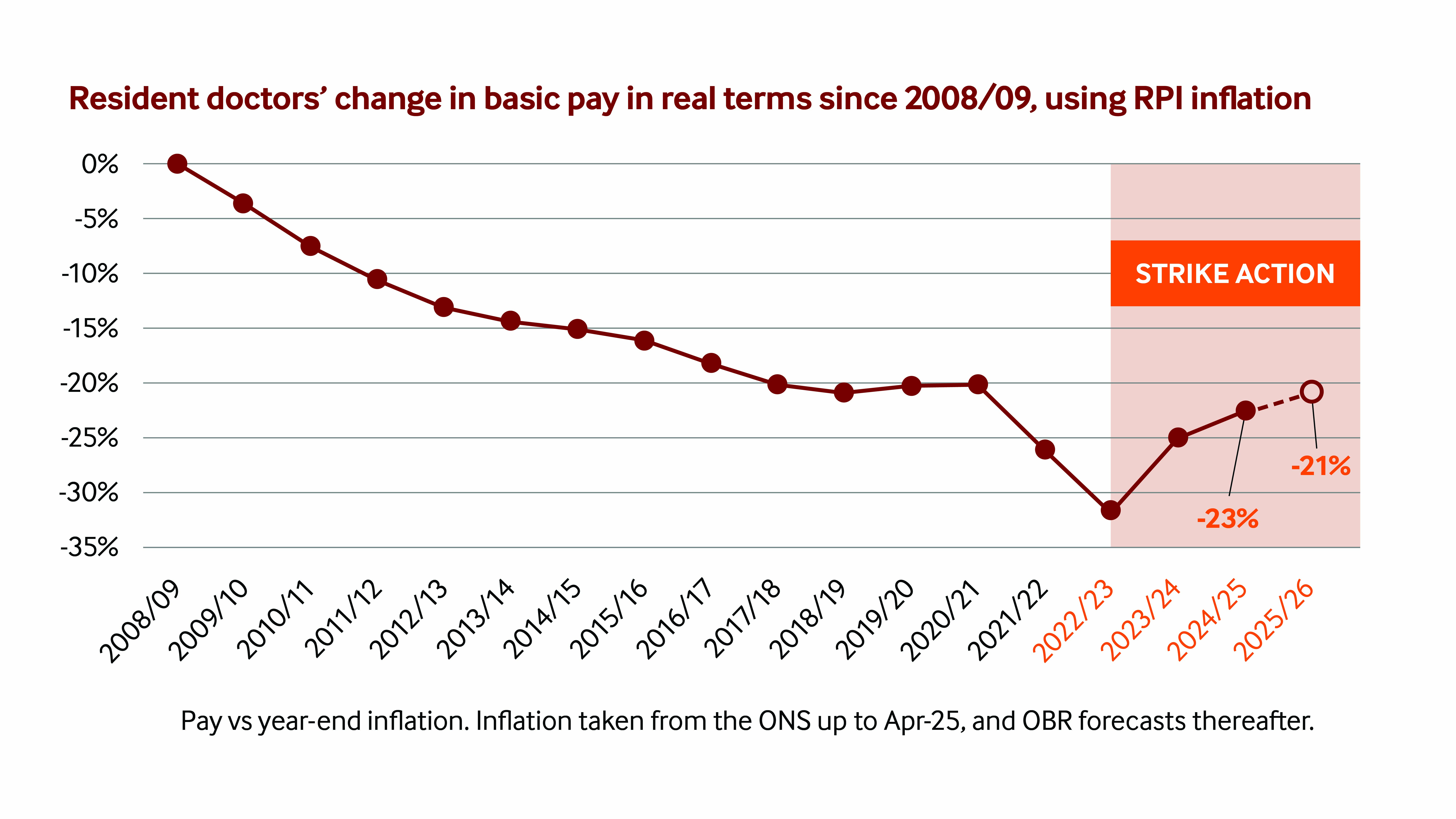
Leaving aside the politics and ethics of the industrial action, it has been noted that the strikes seem to fall on periods of school holidays. But is this really the case?
We can start by listing all the periods of industrial action in England since these strikes started in 2023. Note that the final entry (April 2026) is a future announced strike included because the dates are already fixed; all analyses below treat it alongside completed strikes, which is worth bearing in mind when interpreting results.
library(tidyverse)
library(lubridate)
library(brms)
library(posterior)strikes <- tribble(
~start, ~end,
"2023-03-13", "2023-03-15",
"2023-04-11", "2023-04-14",
"2023-06-14", "2023-06-16",
"2023-07-13", "2023-07-17",
"2023-08-11", "2023-08-14",
"2023-09-20", "2023-09-22",
"2023-10-02", "2023-10-04",
"2023-12-20", "2023-12-22",
"2024-01-03", "2024-01-08",
"2024-02-24", "2024-02-28",
"2024-06-27", "2024-07-01",
"2025-07-25", "2025-07-29",
"2025-11-14", "2025-11-18",
"2025-12-17", "2025-12-21",
"2026-04-07", "2026-04-12"
) %>%
mutate(
start = ymd(start),
end = ymd(end),
length = as.integer(end - start) + 1L
)We can also pull school holidays over this time period for my local authority:
holidays <- tribble(
  ~start,        ~end,          ~label,
  "2023-04-03",  "2023-04-14",  "Spring break 2023",
  "2023-05-29",  "2023-06-02",  "Half-term May 2023",
  "2023-07-22",  "2023-09-03",  "Summer 2023",
  "2023-10-23",  "2023-11-05",  "Half-term Oct 2023",
  "2023-12-23",  "2024-01-03",  "Christmas 2023/24",
  "2024-02-12",  "2024-02-18",  "Half-term Feb 2024",
  "2024-03-29",  "2024-04-14",  "Spring break 2024",
  "2024-05-25",  "2024-06-02",  "Half-term May 2024",
  "2024-07-27",  "2024-09-01",  "Summer 2024",
  "2024-10-19",  "2024-11-03",  "Half-term Oct 2024",
  "2024-12-21",  "2025-01-05",  "Christmas 2024/25",
  "2025-02-15",  "2025-02-23",  "Half-term Feb 2025",
  "2025-03-29",  "2025-04-13",  "Spring break 2025",
  "2025-05-24",  "2025-06-01",  "Half-term May 2025",
  "2025-07-28",  "2025-08-31",  "Summer 2025",
  "2025-10-20",  "2025-10-31",  "Half-term Oct 2025",
  "2025-12-20",  "2026-01-04",  "Christmas 2025/26",
  "2026-02-16",  "2026-02-20",  "Half-term Feb 2026",
  "2026-03-28",  "2026-04-12",  "Spring break 2026"
) %>%
  mutate(start = ymd(start), end = ymd(end))
One important caveat before any analysis: school holidays longer than one week always include weekends, whereas strike days don’t necessarily. This means the overlap metric risks systematically understating the true proportion of working strike days that fell during school holiday weeks, and makes any holiday-targeting effect harder to detect. A more rigorous analysis might restrict both holiday periods and the null distribution to weekdays only.
The simplest analysis would be to just look at the number of strike days that fall on holidays:
# Expand a df with start/end columns to a sorted vector of unique dates
expand_to_days <- function(df) {
  map2(df$start, df$end, seq.Date, by = "day") %>%
    unlist() %>%
    as.Date(origin = "1970-01-01") %>%
    unique() %>%
    sort()
}

# Build a study calendar with logical strike/holiday indicators
build_calendar <- function(strikes_df, holidays_df) {
  study_start  <- min(strikes_df$start)
  study_end    <- max(strikes_df$end)
  strike_days  <- expand_to_days(strikes_df)
  holiday_days <- holidays_df %>%
    filter(end >= study_start, start <= study_end) %>%
    mutate(start = pmax(start, study_start), end = pmin(end, study_end)) %>%
    expand_to_days()

  tibble(date = seq.Date(study_start, study_end, by = "day")) %>%
    mutate(
      is_strike  = date %in% strike_days,
      is_holiday = date %in% holiday_days
    )
}

# Pre-compute all objects needed by permutation functions
prepare_study_objects <- function(strikes_df, holidays_df) {
  cal <- build_calendar(strikes_df, holidays_df)
  list(
    study_start       = min(cal$date),
    study_end         = max(cal$date),
    calendar_df       = cal,
    holiday_vec       = cal$is_holiday,
    strike_vec        = cal$is_strike,
    lengths           = strikes_df$length,
    n_blocks          = nrow(strikes_df),
    total_days        = nrow(cal),
    total_strike_days = sum(strikes_df$length),
    free_days         = nrow(cal) - sum(strikes_df$length)
  )
}
naive_calendar <- build_calendar(strikes, holidays)
naive_summary <- naive_calendar %>%
summarise(
study_days = n(),
strike_days = sum(is_strike),
holiday_days = sum(is_holiday),
strike_holiday_days = sum(is_strike & is_holiday),
pct_days_on_strike = 100 * strike_days / study_days,
pct_days_in_holiday = 100 * holiday_days / study_days,
pct_strike_days_in_holiday = 100 * strike_holiday_days / strike_days
)So during the entire 1127 day period of this dispute, doctors have been on strike for 65 days (6%). Of these, 29% fell during a school holiday — but 27% of all days in the study period were school holidays anyway, so is this really surprising?
One approach might be an exact binomial test. Under a naive null, each strike day has probability equal to the background proportion of holiday days in the study window:
binom.test(
  x = naive_summary$strike_holiday_days,
  n = naive_summary$strike_days,
  p = naive_summary$holiday_days / naive_summary$study_days,
  alternative = "greater"
)
    Exact binomial test

data:  naive_summary$strike_holiday_days and naive_summary$strike_days
number of successes = 19, number of trials = 65, p-value = 0.4048
alternative hypothesis: true probability of success is greater than 0.2724046
95 percent confidence interval:
 0.2006267 1.0000000
sample estimates:
probability of success
             0.2923077
This is non-significant (p = 0.405). However, this approach (and even a simple proportion test) treats each strike day as an independent random draw. In reality, strike days are clustered into a small number of multi-day episodes: a five-day strike is a single scheduling decision, not five independent ones. This breaks the independence assumption, inflates the effective sample size, and can exaggerate significance. The test also ignores calendar structure — the question is whether whole strike blocks were timed to align with holiday periods, not whether individual days happened to land on them.
A better approach is a permutation test that preserves the observed block lengths. We randomly relocate all 15 blocks across the study window many times, and ask: how often do random placements produce as much holiday overlap as was actually observed? This tests whether timing is unusual without assuming independent day-level sampling, and avoids imposing an arbitrary parametric model (binomial, Poisson, hypergeometric) on the strike-scheduling process.
Note that even this model assumes strikes could, under the null, be placed anywhere in the study window with equal probability — including positions that would be implausible given real-world constraints like negotiation timelines, notice periods, postgraduate exams, and clinical rotations.
# Draw a random composition of free_days into (n_blocks + 1) gaps
sample_gaps <- function(free_days, n_blocks) {
  parts <- n_blocks + 1L
  cuts  <- sort(sample.int(free_days + parts - 1L, parts - 1L, replace = FALSE))
  cuts  <- c(0L, cuts, free_days + parts - 1L)
  diff(cuts) - 1L
}

# Total holiday overlap for one random gap arrangement
overlap_from_gaps <- function(gaps, lengths, holiday_vec) {
  pos     <- gaps[1] + 1L
  overlap <- 0L
  for (i in seq_along(lengths)) {
    overlap <- overlap + sum(holiday_vec[pos:(pos + lengths[i] - 1L)])
    pos     <- pos + lengths[i] + gaps[i + 1L]
  }
  overlap
}

# Holiday overlap and strike days restricted to an index window
window_stats <- function(gaps, lengths, holiday_vec, idx_start, idx_end) {
  pos          <- gaps[1] + 1L
  h_overlap    <- 0L
  strike_count <- 0L
  for (i in seq_along(lengths)) {
    bs <- pos; be <- pos + lengths[i] - 1L
    ws <- max(bs, idx_start); we <- min(be, idx_end)
    if (ws <= we) {
      h_overlap    <- h_overlap + sum(holiday_vec[ws:we])
      strike_count <- strike_count + (we - ws + 1L)
    }
    pos <- pos + lengths[i] + gaps[i + 1L]
  }
  c(overlap = h_overlap, strike_days = strike_count)
}

# Full block-preserving permutation test
run_block_permutation_test <- function(strikes_df, holidays_df,
                                       n_sim = 100000, seed = 123) {
  prep <- prepare_study_objects(strikes_df, holidays_df)
  obs  <- sum(prep$holiday_vec[prep$strike_vec])

  set.seed(seed)
  sim_overlap <- replicate(n_sim, {
    gaps <- sample_gaps(prep$free_days, prep$n_blocks)
    overlap_from_gaps(gaps, prep$lengths, prep$holiday_vec)
  })

  tibble(
    study_start      = prep$study_start,
    study_end        = prep$study_end,
    n_blocks         = prep$n_blocks,
    strike_days      = prep$total_strike_days,
    observed_overlap = obs,
    observed_prop    = obs / prep$total_strike_days,
    expected_overlap = mean(sim_overlap),
    expected_prop    = mean(sim_overlap) / prep$total_strike_days,
    p_value          = mean(sim_overlap >= obs),
    null_lo          = quantile(sim_overlap, 0.025),
    null_hi          = quantile(sim_overlap, 0.975),
    sim_overlap      = list(sim_overlap)
  )
}

# Shared histogram helper
plot_overlap_null <- function(sim_vec, observed, subtitle_text, binwidth = 1) {
  tibble(overlap = sim_vec) %>%
    ggplot(aes(x = overlap)) +
    geom_histogram(binwidth = binwidth, boundary = -0.5) +
    geom_vline(xintercept = observed, linetype = "dashed", linewidth = 1) +
    labs(subtitle = subtitle_text, x = "Holiday-overlap days", y = "Count") +
    theme_bw()
}
study_start <- min(strikes$start)
study_end <- max(strikes$end)
recent_start <- study_end %m-% months(18)
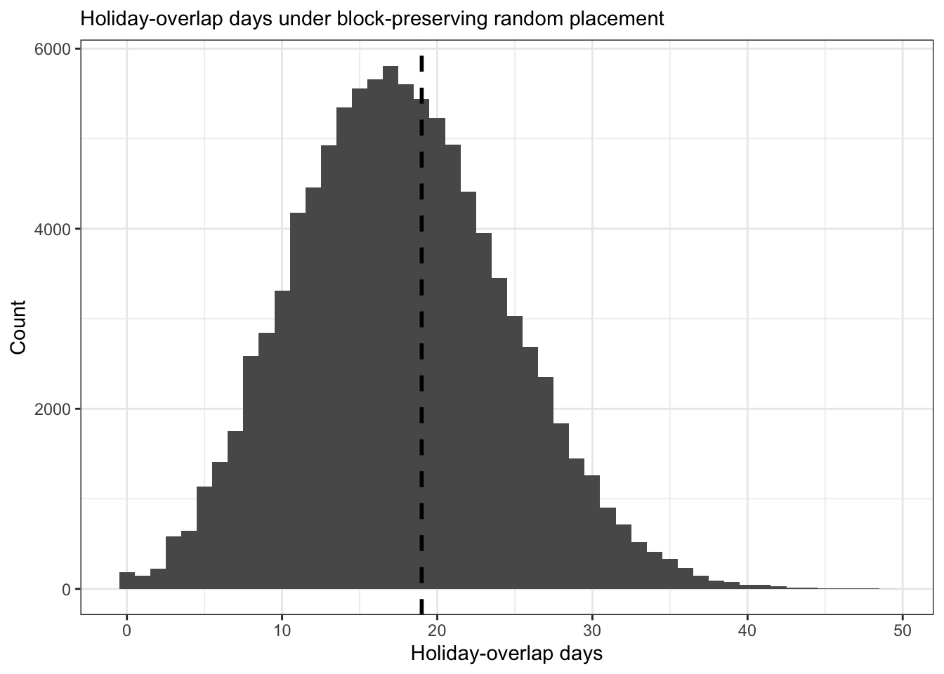
full_result <- run_block_permutation_test(strikes, holidays, n_sim = 100000, seed = 123)Since the start of industrial action, strikes overlapped school holidays on 19 days (29%); random block placement would be expected to produce 17.7 days (27%). This is not significantly higher than chance (p = 0.436):
plot_overlap_null(
  full_result$sim_overlap[[1]],
  full_result$observed_overlap,
  "Holiday-overlap days under block-preserving random placement"
)
A colleague suggested that strike timing may have become more strategic recently. The 18-month cutoff used here was chosen post-hoc in response to that suggestion, which is an important caveat: the analysis should be interpreted as exploratory rather than confirmatory, and the threshold should ideally be pre-specified or subjected to sensitivity analysis (e.g. testing 12- or 24-month windows) to guard against inflated findings from arbitrary splits.
Having said that, let’s run with their suggestion:
strikes_recent <- strikes %>%
filter(end >= recent_start) %>%
mutate(start = pmax(start, recent_start), length = as.integer(end - start) + 1L)
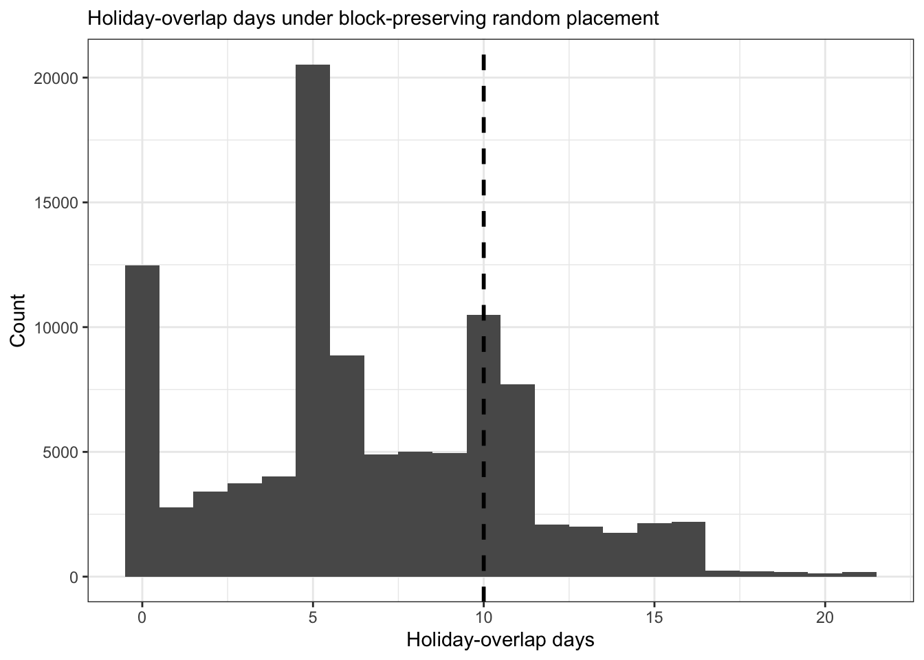
last18_result <- run_block_permutation_test(strikes_recent, holidays, n_sim = 100000, seed = 123)In the last 18 months, 48% of strike days fell in holidays versus an expected 32% (p = 0.293). This is not statistically significant, and given only 4 recent blocks the test has very limited power — a non-significant result here is essentially uninformative.
plot_overlap_null(
  last18_result$sim_overlap[[1]],
  last18_result$observed_overlap,
  "Holiday-overlap days under block-preserving random placement (last 18 months)"
)
Rather than testing each sub-period in isolation (which compounds the low-power problem), we can ask directly whether the recent blocks show more holiday overlap than the earlier ones under the same null model. Note that this contrast is still subject to the same post-hoc cutoff concern above, and we have not corrected for the multiple tests conducted in this section.
run_recent_vs_earlier_contrast <- function(strikes_df, holidays_df,
                                            recent_start, n_sim = 100000, seed = 123) {
  prep <- prepare_study_objects(strikes_df, holidays_df)
  i_r  <- as.integer(recent_start - prep$study_start) + 1L
  i_e  <- i_r - 1L

  # Observed stats computed directly from the calendar vectors
  obs_recent_ov  <- sum(prep$strike_vec[i_r:prep$total_days] & prep$holiday_vec[i_r:prep$total_days])
  obs_recent_sd  <- sum(prep$strike_vec[i_r:prep$total_days])
  obs_earlier_ov <- sum(prep$strike_vec[1:i_e] & prep$holiday_vec[1:i_e])
  obs_earlier_sd <- sum(prep$strike_vec[1:i_e])
  obs_diff       <- obs_recent_ov / obs_recent_sd - obs_earlier_ov / obs_earlier_sd

  set.seed(seed)
  sims <- replicate(n_sim, simplify = "matrix", {
    gaps <- sample_gaps(prep$free_days, prep$n_blocks)
    r    <- window_stats(gaps, prep$lengths, prep$holiday_vec, i_r, prep$total_days)
    e    <- window_stats(gaps, prep$lengths, prep$holiday_vec, 1L, i_e)
    # Use [[ to drop names so c() produces clean column names in the matrix
    p_r  <- if (r[["strike_days"]] > 0) r[["overlap"]] / r[["strike_days"]] else NA_real_
    p_e  <- if (e[["strike_days"]] > 0) e[["overlap"]] / e[["strike_days"]] else NA_real_
    c(p_recent = p_r, p_earlier = p_e, prop_diff = p_r - p_e)
  }) %>% t() %>% as_tibble()

  list(
    obs_recent_prop  = obs_recent_ov  / obs_recent_sd,
    obs_earlier_prop = obs_earlier_ov / obs_earlier_sd,
    obs_diff         = obs_diff,
    p_value          = mean(sims$prop_diff >= obs_diff, na.rm = TRUE),
    sims             = sims
  )
}
contrast <- run_recent_vs_earlier_contrast(strikes, holidays, recent_start, n_sim = 100000, seed = 123)Holiday overlap went from 20% in the earlier period to 48% recently. The difference remains non-significant (p = 0.105), though the wide null distribution reflects the low block counts in each sub-period.
contrast$sims %>%
  ggplot(aes(x = prop_diff)) +
  geom_histogram(binwidth = 0.02, boundary = 0) +
  geom_vline(xintercept = contrast$obs_diff, linetype = "dashed", linewidth = 1) +
  labs(
    subtitle = "Null distribution under block-preserving random placement",
    x = "Recent overlap proportion − earlier overlap proportion",
    y = "Count"
  ) +
  theme_bw()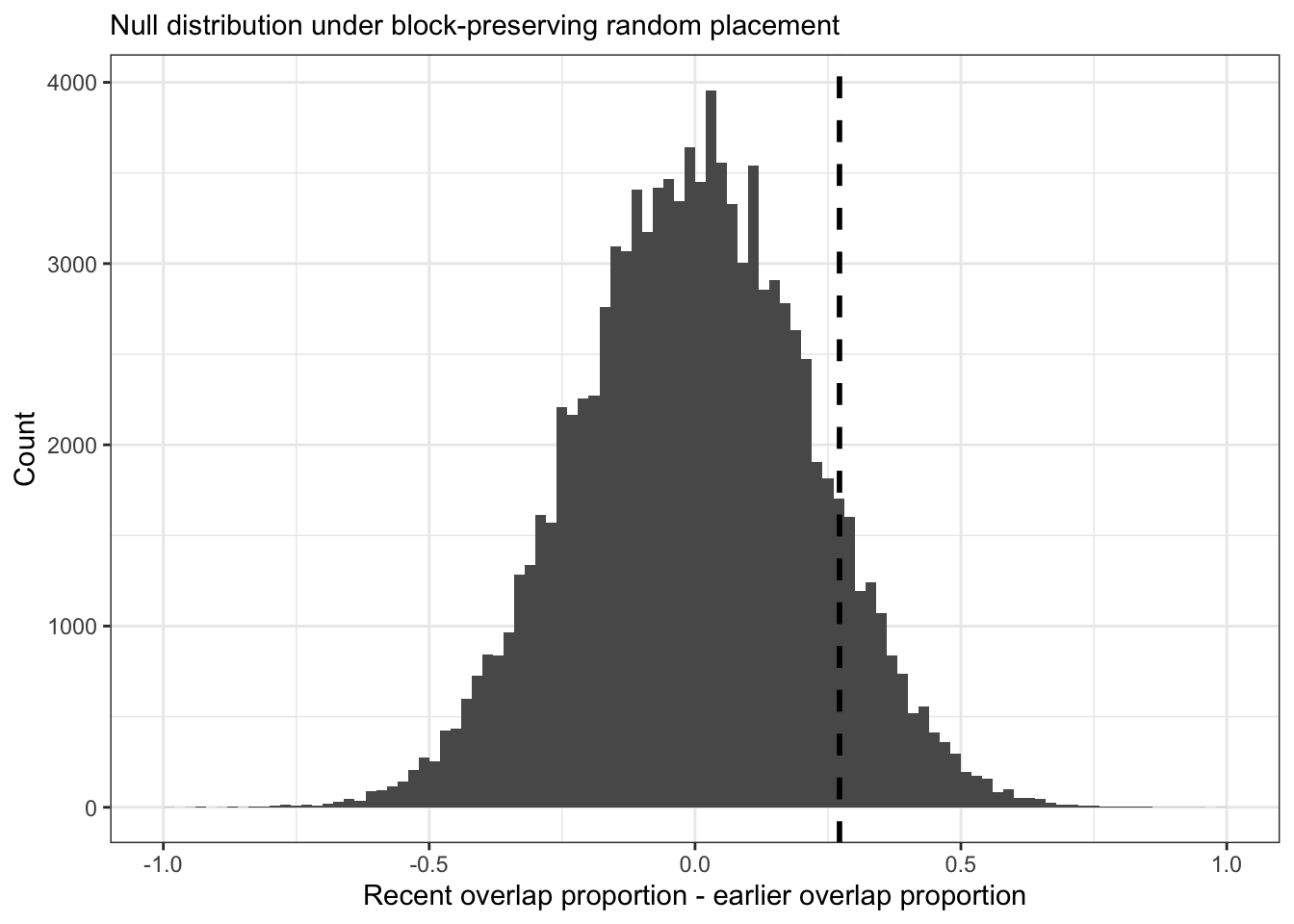
The data suggest a recent shift towards holiday-aligned timing, but under the random-placement null a difference this large still occurs roughly 11% of the time. The result should be read as “weakly suggestive, but not probative” - sure it’s a “non-significant” finding, but the study is probably underpowered anyway, so we’re potentially trying to avoid a type 1 error (setting \(\alpha = 0.05\)) here at the risk of making a type 2 error (unknown \(\beta\)).
When frequentist tests return “non-significant” results with a small dataset at risk of type 2 errors, a Bayesian approach can be more informative: instead of asking \(P(\text{data} \mid H_0)\), we ask what probability the data assign to a genuine recent shift — \(P(\text{recent shift} \mid \text{data})\).
make_block_df <- function(strikes_df, holidays_df, recent_start) {
  study_start  <- min(strikes_df$start)
  study_end    <- max(strikes_df$end)
  holiday_days <- holidays_df %>%
    filter(end >= study_start, start <= study_end) %>%
    mutate(start = pmax(start, study_start), end = pmin(end, study_end)) %>%
    expand_to_days()

  strikes_df %>%
    mutate(block_id = row_number(), recent = as.integer(end >= recent_start)) %>%
    rowwise() %>%
    mutate(
      block_days = list(seq.Date(start, end, by = "day")),
      n_days     = length(block_days),
      n_holiday  = sum(block_days %in% holiday_days)
    ) %>%
    ungroup() %>%
    select(block_id, start, end, length, recent, n_days, n_holiday)
}

extract_posterior <- function(fit, label) {
  as_draws_df(fit) %>%
    transmute(
      model            = label,
      p_earlier        = plogis(b_Intercept),
      p_recent         = plogis(b_Intercept + b_recent),
      risk_diff        = p_recent - p_earlier,
      risk_ratio       = p_recent / p_earlier,
      odds_ratio       = exp(b_recent),
      recent_gt_earlier = p_recent > p_earlier
    )
}

summarise_posterior <- function(draws) {
  draws %>%
    group_by(model) %>%
    summarise(
      across(c(p_earlier, p_recent, risk_diff, risk_ratio, odds_ratio),
             list(mean = mean,
                  lo   = \(x) quantile(x, 0.025),
                  hi   = \(x) quantile(x, 0.975))),
      pr_recent_gt_earlier = mean(recent_gt_earlier)
    ) %>%
    ungroup()
}
We use a beta-binomial model because we have only 15 strike blocks (too few for a standard binomial regression to be reliable), between-block variability in overlap probability is plausible, and the model explicitly allows each block its own true overlap probability varying around a group mean, rather than forcing all blocks to share one fixed probability. With only 4 recent and 11 earlier blocks, however, the model is working with very sparse data and the resulting credible intervals will be wide.
For block \(i\), the number of holiday-coincident strike days \(Y_i \sim \text{Beta-Binomial}(n_i, \mu_i, \phi)\), where \(\text{logit}(\mu_i) = \alpha + \beta \cdot \text{Recent}_i\). We will use weakly informative priors (\(\alpha \sim \mathcal{N}(0, 1.5)\), \(\beta \sim \mathcal{N}(0, 1)\), \(\phi \sim \text{Exponential}(1)\)) i.e. we don’t have any expectation on what we’ll find:
block_df <- make_block_df(strikes, holidays, recent_start)

fit_bb <- brm(
  n_holiday | trials(n_days) ~ recent,
  data    = block_df,
  family  = beta_binomial(),
  prior   = c(
    prior(normal(0, 1.5), class = "Intercept"),
    prior(normal(0, 1),   class = "b"),
    prior(exponential(1), class = "phi")
  ),
  chains  = 4, iter = 4000, warmup = 1000,
  seed    = 123, refresh = 0
)

print(summary(fit_bb))
Family: beta_binomial
Links: mu = logit
Formula: n_holiday | trials(n_days) ~ recent
Data: block_df (Number of observations: 15)
Draws: 4 chains, each with iter = 4000; warmup = 1000; thin = 1;
total post-warmup draws = 12000
Regression Coefficients:
Estimate Est.Error l-95% CI u-95% CI Rhat Bulk_ESS Tail_ESS
Intercept -1.10 0.54 -2.20 -0.07 1.00 9892 8567
recent 0.65 0.72 -0.78 2.08 1.00 11412 8532
Further Distributional Parameters:
Estimate Est.Error l-95% CI u-95% CI Rhat Bulk_ESS Tail_ESS
phi 0.57 0.37 0.12 1.54 1.00 10153 7796
Draws were sampled using sampling(NUTS). For each parameter, Bulk_ESS
and Tail_ESS are effective sample size measures, and Rhat is the potential
scale reduction factor on split chains (at convergence, Rhat = 1).draws_bb <- extract_posterior(fit_bb, "Beta-binomial")
smry <- summarise_posterior(draws_bb)The posterior estimates the holiday overlap probability as 26.1% (95% CrI 10–48.2%) for earlier strikes and 39.8% (14.2–69.4%) for the last 18 months:
draws_bb %>%
  select(p_earlier, p_recent) %>%
  pivot_longer(everything(), names_to = "period", values_to = "prob") %>%
  mutate(
    period = recode(period, p_earlier = "Earlier strikes", p_recent = "Last 18 months"),
    prob   = 100 * prob
  ) %>%
  ggplot(aes(x = prob, fill = period)) +
  geom_density(alpha = 0.4) +
  labs(
    subtitle = "Posterior probability that a strike day fell in a school holiday",
    x = "Probability (%)", y = "Density", fill = NULL
  ) +
  theme_bw()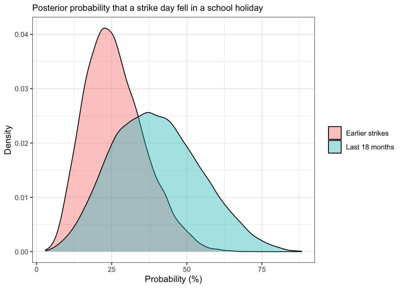
The absolute increase is 13.7% (95% CrI -15 to 44.1), with a relative risk of 1.71 (0.57–3.94). The posterior probability that recent overlap exceeded earlier overlap was 82.1%:
dens_df <- density(draws_bb$risk_diff, n = 2000) %>%
  with(tibble(x = x, y = y, positive = x > 0))

ggplot(dens_df, aes(x = 100 * x, y = y)) +
  geom_area(data = filter(dens_df, !positive), alpha = 0.35) +
  geom_area(data = filter(dens_df,  positive), alpha = 0.75) +
  geom_vline(xintercept = 0, linetype = "dashed", linewidth = 1) +
  annotate(
    "text",
    x     = 100 * mean(draws_bb$risk_diff),
    y     = max(dens_df$y) * 0.9,
    label = paste0("Pr(recent > earlier) = ",
                   scales::percent(mean(draws_bb$recent_gt_earlier), accuracy = 0.1)),
    vjust = 0
  ) +
  labs(
    subtitle = "Shaded area to the right of 0 is the posterior probability of a genuine increase",
    x = "Recent minus earlier overlap probability (percentage points)",
    y = "Posterior density"
  ) +
  theme_bw()
A Pr(recent > earlier) of 82.1% means the posterior is moderately in favour of a real increase, but far from conclusive. It is tempting to read this as “there’s a 17.9% chance there’s nothing there”, but that framing imports a hypothesis-testing mindset into a quantity that is really just a posterior summary — the wide credible intervals are the more informative take-home. Given that the model is fitting on only 15 blocks with a post-hoc period split, the uncertainty is appropriate.
Overall, these analyses suggest that English resident doctor strikes have overlapped school holidays more often than would be expected from a naive day-level comparison, but the signal weakens substantially once calendar structure is modelled properly.
In the block-preserving permutation analyses, full-period overlap appeared only marginally above chance, and the recent-versus-earlier comparison suggested increasing holiday alignment in the most recent period without that difference being statistically unusual under the random-placement null. The Bayesian model pointed in the same direction, estimating higher recent overlap but with wide credible intervals once between-block heterogeneity was accounted for.
Several limitations are worth keeping in mind across all analyses. First, the 18-month recent/earlier split was chosen post-hoc in response to a colleague’s suggestion; any inference about a temporal trend is therefore exploratory and would need to be confirmed in a pre-specified analysis or with sensitivity analyses across alternative cutpoints. Second, the permutation null assumes strike blocks could have been placed anywhere in the study window with equal probability, which ignores real constraints (notice periods, negotiations, exams, clinical rotations, political timing). Third, many of the school holidays include weekends, whereas the initial round of strikes were predominantly weekdays. A cleaner analysis would restrict both the overlap metric and the null distribution to weekdays. Finally, the Bayesian model is fitting relatively sparse data (15 blocks, 4 of them recent), so the posterior estimates carry substantial uncertainty that the point summaries can obscure.
Taken together the results are consistent with some evidence of increased holiday alignment in the more recent period, but do not provide strong grounds for a confident claim of deliberate targeting. These findings speak to whether observed timing looks unusual relative to a simplified chance model; they say nothing about intent, strategy, or political motivation. Having said this industrial action is, by design, intended to cause maximum disruption — and coincidence with school holidays, when consultant cover is already stretched by childcare and travel, would not be an unreasonable tactic even if the statistical evidence here remains equivocal.