Handwashing for the avoidance of COVID-19: A Bayesian Meta Analysis
Rev Bayes says: Keep washing your hands!

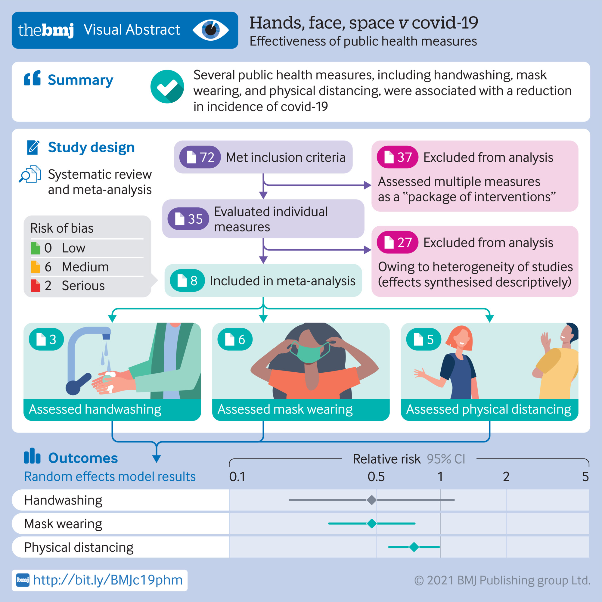
We’ve all had enough of this buffoon spouting rubbish for the last two years - but does the “Hands / Face / Space” message he promoted in lieu of actual governance or action have an evidence base? That’s the question that Talic et al tried to answer in their BMJ article this week, and presented their results with an elegant infographic:
The raw (limited) data on handwashing looks like this:
| Study | COVID+ handwashers | All handwashers | COVID+ non-handwashers | All non-handwashers | RR (95% CI) | Comments |
|---|---|---|---|---|---|---|
| Doung-Ngern 2020 | 52 | 424 | 158 | 612 | 0.34 (0.13 to 0.88) | Used “always” vs “sometimes/never” |
| Lio 2021 | 12 | 975 | 12 | 162 | 0.30 (0.11 to 0.81) | |
| Xu 2020 | 51 | 7895 | 6 | 263 | 0.58 (0.40 to 0.84) | Wrong reference in the article! |
We’ll use the excellent {bayesmeta} package to analyse this. Firstly build a table of log-RR using the {metafor} package:
data.es <- metafor::escalc(measure="RR",
                   ai = hw_cases,  n1i = hw_total,
                   ci = nhw_cases, n2i = nhw_total,
                   slab = Study, data = raw_data)
Now lets perform a Bayesian random-effects meta-analysis, assuming a minimally-informative prior, and plot the results:
ma01 <- bayesmeta::bayesmeta(y = data.es[, "yi"],
                             sigma = sqrt(data.es[, "vi"]), # Convert variance to standard error
                             labels = data.es[, "Study"],
                             mu.prior.mean = 0, mu.prior.sd = 4,
                             tau.prior = function(t) bayesmeta::dhalfcauchy(t, scale = 0.5)
                             )

bayesmeta::forestplot.bayesmeta(ma01, exponentiate=TRUE)

As with a frequentist meta-analysis, this shows the estimated relative risks of each study along with the 95% confidence intervals of the standard errors, but additionally in grey the shrinkage intervals for each study, i.e. the posterior given each study’s effects on our minimally-informative prior. At the bottom the plot shows the 95% credible intervals for the effect (in this case handwashing has a relative risk of 0.33 for catching COVID-19, with a 95% credible interval of 0.15 to 0.63), and for the predictive distribution (0.34, 0.08 to 1.12), i.e. 95% of our unobserved values of the RR from handwashing in future studies will lie between 0.08 and 1.12, given the data we have so far.
This allows us to calculate the probability of handwashing having a non-beneficial effect:
1 - ma01$pposterior(mu = 0)
## [1] 0.01111698
i.e. handwashing is 98.9% likely to reduce the risk of catching COVID-19. For an essentially free intervention, I have sufficient belief in it to keep going!
With that in mind, let’s plot the posterior distribution, i.e. the strength of our belief in handwashing, given the data from the three studies meta-analysed:
x <- seq(-3.5, 0.25, length=200)

library(ggplot2)

ggplot() +
  aes(x = exp(x), y = exp(ma01$dposterior(mu = x))) +
  geom_line() +
  geom_vline(xintercept = 1.0, lty = "dashed") +
  xlab("Relative risk") +
  ylab("Posterior density") +
  theme_bw()
 Obviously this needs to be sensitivity tested with other distributions, etc, but hopefully this quick analysis demonstrates the power of a Bayesian analysis (how likely something is, given the data we have) over a frequentist approach (how likely the data is, assuming there is no effect).
Nick Plummer
Trainee anaesthestist intensivist, amateur data scientist, slow triathlete
Recovered geophysicist. Cares intensively, sciences data, and occasionally gives an anaesthetic.