Coin flips and Bayesian reasoning

One final gasp of usefulness from Twitter

Last updated on Sep 1, 2024 5 min read

Everyone is abandoning ship from ~~Twitter~~X to Bluesky (come join me there!). However, it’s not quite yet entirely porn-bots and right wing extremism - there’s still some excellent posts, like this one:

So what’s the answer?

We want to find $P(C_R ∣ D)$ i.e., the probability that the coin is rigged given the data (10 heads in a row). To calculate this, we use Bayes’ theorem:

$$P(C_R ∣ D) = \frac{P(D | C_R) P(C_R)}{P(D)}$$

Where:

$P(D | C_R)$ is the probability of getting 10 heads if the coin is rigged (i.e. 1)
$P(C_R)$ the probability the coin is rigged before any data is known (1/10,000)
$P(D)$ the marginal probability of getting 10 heads.

This last one is a bit more complex to work out, as it’s all the ways we can get 10 heads:

$$P(D)=P(D∣C_R) P(C_R) +P (D∣C_F) P(C_F)$$

i.e. the probability of getting it if the coin is rigged times the probability that the coin is rigged, plus the probability of getting if if the coin is fair ( $\left( \frac{1}{2} \right) ^ 2 = 1/1024$ ) times the probability that the coin is fair (9,999/10,000).

So sticking all these numbers together gives us:

P_Cr = 1/10000
P_Cf = 1-P_Cr

P_D_Cr = 1
P_D_Cf = (1/2)^10

P_D = P_D_Cr*P_Cr + P_D_Cf*P_Cf

P_Cr_D = (P_D_Cr * P_Cr) / P_D
P_Cf_D = (P_D_Cf * P_Cf) / P_D

P_Cr_D * 100 # Value in percent

## [1] 9.289667

Despite the ten heads, the coin only has a 9% chance of being rigged given the sheer number of unrigged coins. Was this what you intuitively thought?

How many flips does it take?

The follow up question then is - how many flips do we need to be sure? Well, not sure, but “on the balance of probabilities” we think that the coin is rigged?

To answer that we need to find the number of consecutive heads $n$ such that $P(C_R|D_n) > P(C_F|D_n)$. We can do this by expanding the inequality:

$$ \frac{P(D_n|C_R) P(C_R)}{P(D_n|C_F) P(C_F)} > 1$$

Since $P(D_n|C_R)$ is always 1, and $P(D_n|C_F) = \left( \frac{1}{2} \right) ^ n$, this simplifies down to $9999 \times \left( \frac{1}{2} \right) ^ n <1$ i.e. $n > \frac{log(9999)}{log(2)} > 13.3$. So if you get any more than 14 heads, this suggests the coin is probably rigged.

What this demonstrates is how Bayesian thinking works - we update our prior probabilities with new data to generate posterior probabilities. Every time we flip another heads, the posterior likelihood of the coin becoming rigged becomes slightly higher - let’s demonstrate this graphically with a simulations:

library(tidyverse)

# Starting parameters
total_coins <- 10000
rigged_prob <- 1 / total_coins
fair_prob <- 9999 / total_coins

# Update posterior probabilities after observing heads
update_posterior <- function(current_posterior_rigged, current_posterior_fair, is_head) {
  if (is_head) {
    likelihood_rigged <- 1  # Rigged coin always gives heads
    likelihood_fair <- 0.5  # Fair coin has 50% chance of heads
  } else {
    likelihood_rigged <- 0  # Rigged coin cannot give tails
    likelihood_fair <- 0.5  # Fair coin has 50% chance of tails
  }
  
  posterior_rigged <- likelihood_rigged * current_posterior_rigged
  posterior_fair <- likelihood_fair * current_posterior_fair
  
  total_posterior <- posterior_rigged + posterior_fair
  if (total_posterior == 0) {
    return(c(0, 1))  # Edge case where both posteriors are zero
  }
  return(c(posterior_rigged / total_posterior, posterior_fair / total_posterior))
}

# Simulate 20 flips and update the posterior probabilities
n_flips <- 20
posterior_probs_rigged <- numeric(n_flips)
posterior_probs_fair <- numeric(n_flips)
current_posterior_rigged <- rigged_prob  # Start with prior probability for rigged coin
current_posterior_fair <- fair_prob      # Start with prior probability for fair coin

for (flip in 1:n_flips) {
  # Simulate a flip observing heads
  is_head <- TRUE
  
  # Update the posterior probabilities
  posteriors <- update_posterior(current_posterior_rigged, current_posterior_fair, is_head)
  current_posterior_rigged <- posteriors[1]
  current_posterior_fair <- posteriors[2]
  
  posterior_probs_rigged[flip] <- current_posterior_rigged
  posterior_probs_fair[flip] <- current_posterior_fair
}

# Save this in a data frame for plotting
posterior_df <- data.frame(
  Flip = 1:n_flips,
  Posterior_Rigged = posterior_probs_rigged,
  Posterior_Fair = posterior_probs_fair
)

ggplot(posterior_df, aes(x = Flip)) +
  geom_line(aes(y = Posterior_Rigged, color = "Rigged Coin"), size = 1) +
  geom_point(aes(y = Posterior_Rigged, color = "Rigged Coin"), size = 2) +
  geom_line(aes(y = Posterior_Fair, color = "Fair Coin"), size = 1) +
  geom_point(aes(y = Posterior_Fair, color = "Fair Coin"), size = 2) +
  geom_hline(yintercept = rigged_prob, linetype = "dashed", color = "gray", size = 1, label = "Prior Probability (Rigged)") +
  geom_hline(yintercept = fair_prob, linetype = "dashed", color = "gray", size = 1, label = "Prior Probability (Fair)") +
  labs(title = "Posterior Probability of Coin Being Rigged vs Fair After Each Flip",
       x = "Number of Flips",
       y = "Posterior Probability",
       color = "Coin Type") +
  theme_bw() +
  theme(legend.position = "bottom")

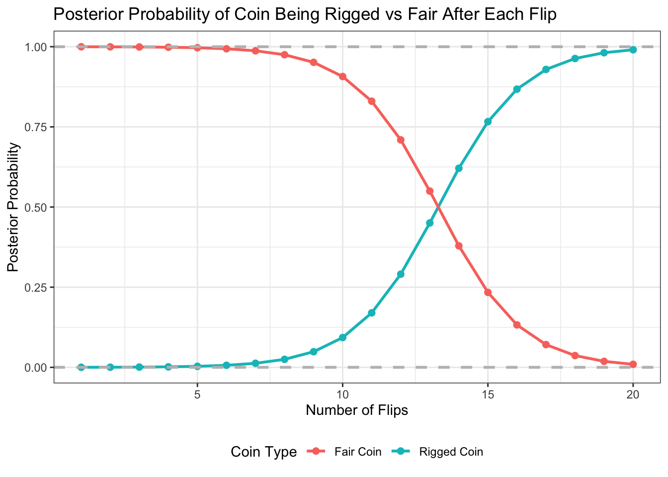
The dashed line at the top is the prior probility of the coin being fair (9,999/10,0000) and the bottom the prior probability of the coin being rigged (essentially zero). As the number of flips increases, the probabilities slowly converge - up to that key point that we calculated above at 13 to 14 flips on heads where the probabilities switch. Any more than that and it becomes more and more likely that the coin is rigged.

But there’s more

Professor Litt wasn’t done yet:

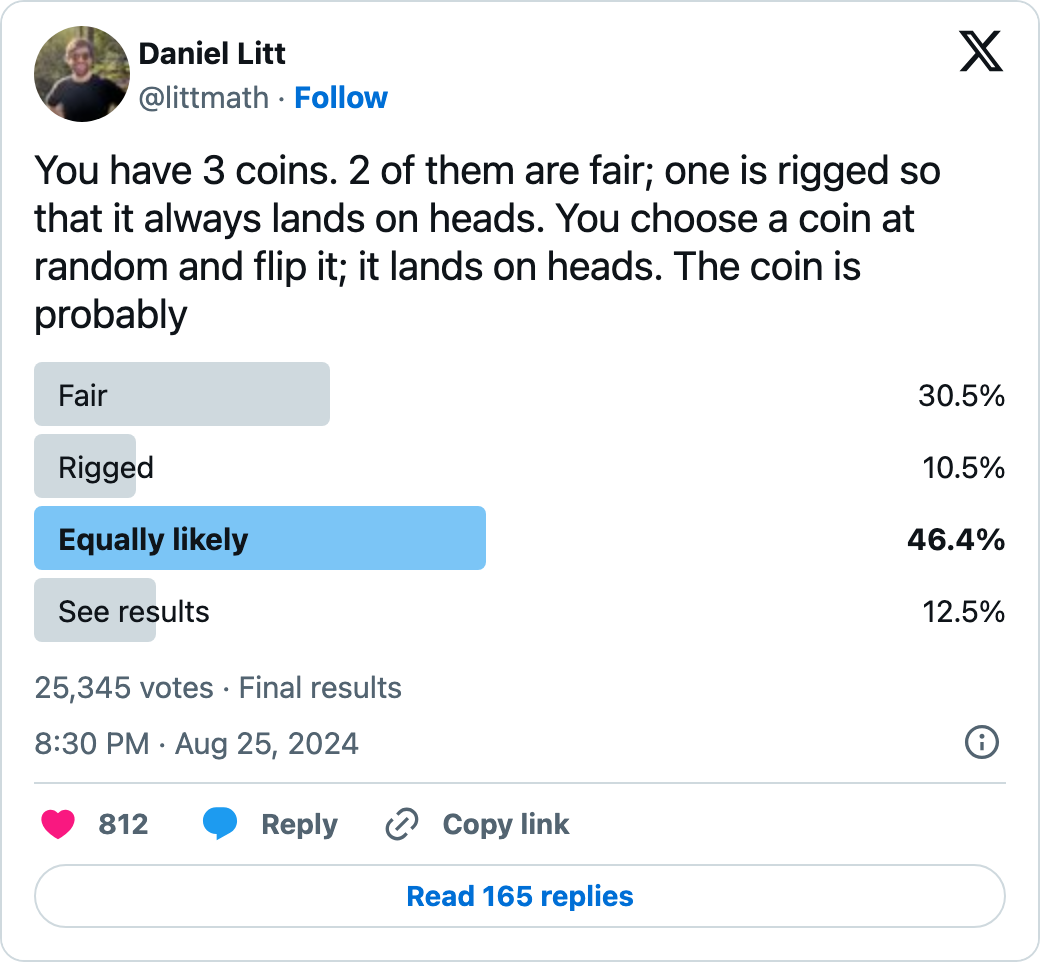
What’s the intuitive answer?

Let’s do the maths again:

P_Cr = 1/3
P_Cf = 1-P_Cr

P_D_Cr = 1
P_D_Cf = (1/2)#^1

P_D = P_D_Cr*P_Cr + P_D_Cf*P_Cf
# i.e. P_D = 1/3 + 1/3 = 2/3

P_Cr_D = (P_D_Cr * P_Cr) / P_D
P_Cf_D = (P_D_Cf * P_Cf) / P_D

P_Cr_D * 100 # Value in percent

## [1] 50

So after one flip resulting in heads, the coin is equally likely to be rigged or fair.

I have to admit this one caught me out.

statistics

Coin flips and Bayesian reasoning

So what’s the answer?

How many flips does it take?

But there’s more

Nick Plummer

Trainee anaesthestist intensivist, amateur data scientist, slow triathlete