Bayesian Statistics for Doctors

REMAP-CAP have released their preliminary report into immune modulation and everyone is getting very excited by the potential for tocilizumab and sarilumab to improve COVID-19 outcomes in critical care. You even go so far as to think it would make a great journal club paper… until you read the methods section:

The primary analysis was generated from a Bayesian cumulative logistic model, which calculated posterior probability distributions of the 21-day organ support-free days (primary outcome) based on evidence accumulated in the trial and assumed prior knowledge in the form of a prior distribution

It’s not that bad, honest. Let’s take a deep breath and talk statistical inference for doctors and, borrowing heavily from Daniel Laken’s excellent Coursera, consider how we do it in terms of yoga:

Karma: the Path of Action

The frequentist approach to statistics is the “classical” one we’re all taught at medical school. We do a null-hypothesis significance test (NHST), apply a statistical test, and the lower the p-value, the better the stats, right?

Afraid not.

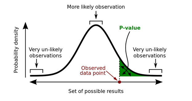
This type of statistics tells us about the outcome of experiments in the long run, but actually tells us nothing about the current test. The p-value is nothing but a measure of how surprising the data we have is, assuming there’s no true effect (i.e. that the null hypothesis is true). It doesn’t tell us anything about the alternative hypothesis, least of all how certain it is.

All of medical statistics is essentially seeing if there’s a difference in something between two populations - e.g. is there a height difference between men and women, or do people with COVID given tocilizumab live longer than people who don’t. Let’s call this the effect size. The most accurate way to calculate this would be to measure the parameter of interest in everyone in these two populations, but that’s an impossible ask: measuring all the men and women in the world is clearly impossible, and although we can measure outcomes for all the COVID patients given tocilizumab so far, we need to be able to generalise this to all the people we want to give it to.

So the next best option is to measure the effect in a sample taken from the population of interest, then use a statistical test to guess how likely the effect size - averaged over everyone we’ve measured - is to apply to the population(s) of interest. This is a function of the mean effect size $\overline x$, the standard deviation in our measurements $\sigma$ (variation in our measured effect size), and the number of people we’ve looked at ($n$). The difference (potential effect size) between the groups in this case is almost never zero, so we need to determine if this is a real signal, or if it’s random noise due to how we’ve chosen our samples. That’s where the p-value comes in.

The NHST-way to calculate this is to plug the $\overline x$, $\sigma$, and $n$ into a formula for that particular test statistic, compare this against a known distribution, and measure how different this result is compared to the distribution we’d expect if there was no true effect (the null hypothesis H0):

The key thing to remember here is that the p-value is the probability of the data given H0 is true, not the probability of the theory (H1, the alternative hypothesis, which is simply “there is a difference”) being “true”, or indeed of H0 being false. It’s a guide to the behaviour of the test in the long run - if you sample n people again and again from these populations, you won’t be wrong more than $\alpha$ of the time, and we commonly set $\alpha = 0.05$ in medical statistics (i.e. 1:20 chance of the data not being surprising) as “significant”. Why is this?

These graphs show the p-values for 100,000 simulated experiments, each time drawing $n=26$ samples. To the left, there is no real difference - population mean is 100, compared to a hypothesis (H0) mean of 100. Because there’s no real effect the p-values are uniformly distributed, yet you can see that 5% of the time the p-values are still < 0.05 (i.e. an error rate of $\alpha$. To the right, the population mean is instead 110, so the p-value distribution is skewed towards there being a real signal (or an error rate of $< \alpha$, with the exact shape of the distribution also depending on the power of the test). But still, all we can say from this is that it’s highly likely that the data is improbable given there being no real effect, or in stats speak:

$$P(data | H_{0}) \leq 0.05$$

From this if $p \leq \alpha$ we conclude the data is (probably) not noise, and if $p > \alpha$ we remain uncertain if the data is noise (although most authors will say “it is noise”, unless they’re trying to push a different agenda, see below…)

Jnana: the Path of Knowledge

In most uses of NHST medical statistics, we should stop there. Unfortunately many authors will draw an inference from that probability of data to try and say something about our hypothesis (even though we can’t without using Bayesian statistics, more on this later). Worse still, we often draw inferences from our probability of data to say something that we’ve a priori said we can’t! How many times do you read “there was a trend towards” when the data has failed the pre-specified significance test?! Please stop doing this.

If we want to say more (like “trends”, which is really trying to make a statement on the strength in our convictions regarding a hypothesis) we need to move from describing the data given purely the null hypothesis (there being no difference), to talking about the likelihood of different hypotheses being true, given said data. This is where Richard Royall’s likelihood paradigm comes in.

Each hypothesis has a potential set of parameters for the data - mean, variation, etc. Lets call these $\theta$. So we can work out a likelihood of the data given each potential hypothesis, $L(\theta)$, which on its own is fairly meaningless, but when compared to another likelihood (for example likelihood under H1 vs likelihood under H0) gives us a likelihood ratio (LR).

Royall defined LR > 8 as moderately strong evidence for H1, and LR > 32 as strong evidence for H1, but likelihoods are simply relative evidence - just because data is more likely under one hypothetical distribution than another doesn’t mean that it has come from either of them, just that there is more relative evidence for one than another (while they could both still be highly unlikely). To say more about where the data has come from we need Reverend Bayes and his probability theorem.

Bhakti: the Path of Belief

Bayesian statistics allows us to compare the likelihood of different hypotheses given the data, and use these to modify our belief in each of those hypotheses. It all relies on Bayes’ theorem and the probabilities we’ve observed to calculate the probability of out hypothesis being true, given the data we’ve seen, and what we think we know about it (and the strength of that knowledge):

$$ P(H | data ) = \frac{P(data | H) P(H)}{P(data)} $$

The beauty of Bayesian thinking is that our degree of belief in our hypothesis depends on our prior knowledge and experience (blue curve), but each time we add data (red dots) their corresponding likelihood distribution (red curve) alters our subsequent (“posterior”) belief (purple curve), which in turn becomes the prior for the next set of data:

$$ P(posterior) = LR * P(prior)$$

I find it very strange that, on the whole, doctors don’t get Bayesian statistics because this is exactly how clinical reasoning works:

• Lets say you’re in A&E, and you’re told someone has chest pain. You already have a guess that this might be an MI, and that depends on where you work and it’s demographics, degree of deprivation, etc. That’s your prior.
• Now you set eyes on the patient, and they’re an overweight, middle-aged man, clammy and clutching at their chest. Your likelihood of this being a MI versus anything else is relatively high, so you update your posterior to be an even higher probability.
• You’re handed an ECG. It’s essentially normal. LR for hypothesis-MI based on this this is pretty low, but your prior (posterior from the last step) is still stonkingly high, so your new posterior given this new info is still reasonably sporting.
• The troponin comes back at 10,000. Very high LR, so your new posterior is so high that it’s essentially certain. You call cardiology and move onto the next patient.

(As an aside the NNT is a brilliant website which actually has all these LRs for various conditions, and similar analyses of treatments.)

Bayesian statistics is the process of applying this type of thinking to trial data. Instead of setting an end-point (“once we’ve recruited x people, according to our power calculation…”) and then doing a one-off test to regarding the data (“our p-value was…”), a Bayesian trial updates the relative probabilities of the hypotheses being true every time a new piece of data is added, resulting in a “credible interval” of reasonably probable parameters for the true distribution (holding the data fixed, and varying $\theta$, whereas “confidence intervals” of NHST imagine that the parameter $\theta$ has one true, but unknown, value). Over time as more and more data is added the credible interval narrows until the result becomes sufficiently certain to declare, announcing the most credible values of $\theta$, i.e. the effect size.

$$ \frac{P(H_{1} | D)}{P(H_{0} | D)} = \frac{P(D | H_{1})}{P(D | H_{0})} * \frac{P(H_{1})}{P(H_{0})}$$

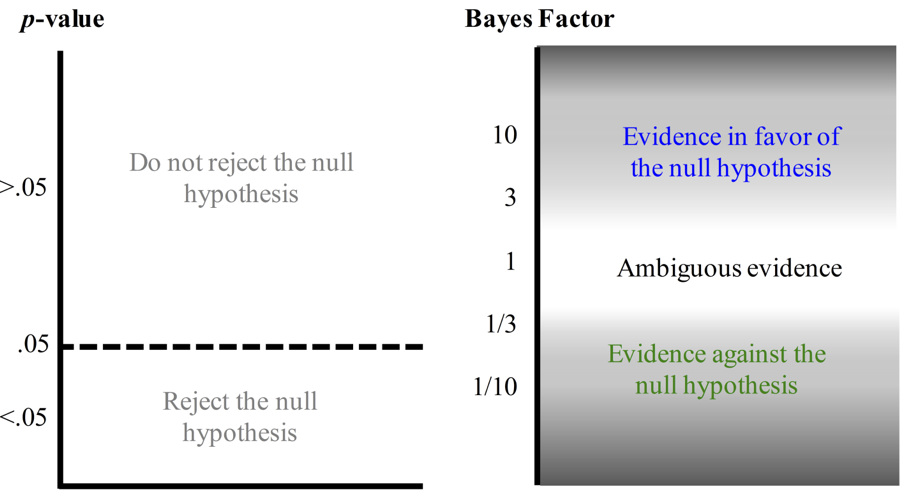
If you’re desperate for a p-value, the other way to use Bayesian stats is to think of the Bayes Factor $P(D | H_{1}) / P(D | H_{0})$ (essentially the LR incorporating any pre-existing information) as analogous to the p-value, but instead of having an arbitrary cut off at $\alpha$ defining “significance” of the data, giving varying weights to the two competing hypotheses:

The most complicated part of all this to get your head around is the prior distributions, as clearly choosing different ones of these could potentially lead to huge differences in posterior distributions, at least initially? Well that’s actually one of the major strengths of Bayesian analyses, as you can set different priors and collect data until they converge on something meaningful. Trials will usually report results given a null prior (i.e. no odds of their being anything meaningful), a neutral prior (no difference), an optimistic prior (as one would use for a power calculation in NHST), and a pessimistic prior (the opposite to what you hope to find). For example see this figure from the Bayesian reanalysis of the ANDROMEDA-SHOCK trial:

What does this all mean for REMAP-CAP?

REMAP-CAP is brilliant. It’s the adaptive platform trial stats nerds like me have been waiting for in critical care, and landed at the right time and place to be able to add domain after domain to study the COVID-19 pandemic in addition to its intended target of community acquired pneumonia. Patients get randomised across multiple domains, which can be added or removed without major changes to the running of the trial, and the analysis allows interactions between these domains to be picked out an adjusted for, with sequential Bayesian analyses within domains not only until a signal is found, but also (and this is the coolest bit) adjusting the probability with which interventions are delivered to patients as evidence is found to support them (after each “adaptive analysis”). In essence, if everyone was recruited to the study, there would be no need to announce the results, because the study mechanics would put people on the therapies with the best evidence for them automatically as that evidence becomes stronger and stronger. Yeah, I know. Awesome, right?

If you’re interested (and why wouldn’t you be in the future of clinical research?) CCR has put together a series of great podcasts on REMAP-CAP, and as always The Bottom Line have a great summary of the initial results regarding steroids.

Want even more?

If you’re keen for more details, Scholarpedia has a great article on Bayesian stats in much more depth (which I’m mostly linking to because I have an academic man-crush on David Spiegelhalter) and Eoin Travers has a lovely article on the maths of frequentist and Bayesian hypothesis testing if you’re really getting into it. From a more clinical point of view there’s a good BJA Education article and review from BJA worth checking out (which are also potential FRCA/FFICM fodder, be warned!).